21 Dec 2020 The Mortgage-Implied Illiquidity Premium
The determination of the illiquidity premium that is applicable in the valuation of an equity release mortgage is, arguably, the most contentious aspect of the valuation of the asset. To be sure, there are many other aspects of the valuation of this complex and illiquid asset that are difficult, that require judgment and where it must be accepted that there is some inevitable uncertainty in the accuracy of the assumptions.
Borrower prepayment behaviour is a good example of an important and inherently uncertain aspect of the mortgage valuation basis. Equity release mortgage valuation practices have perhaps been notably unusual in the degree to which they have assumed that granting the borrower a unilateral option results in an asset that is less risky and more valuable to the lender[1].
The deferment rate and the volatility of the underlying asset are two further obvious examples. However, unlike the illiquidity premium, these two variables do not affect the valuation of the pre-NNEG component of the asset, and so, for a given set of prices and a given pre-NNEG valuation basis, these two variables cannot (jointly) impact on the NNEG valuation. That is, if calibrating a valuation basis to an observed ERM price, the total size of that asset’s NNEG is determined by the difference between the given price and the pre-NNEG valuation; and the pre-NNEG valuation, which is merely valuing some fixed cashflows, does not depend on the deferment rate or volatility; therefore, a change in either deferment rate or house price volatility must imply a change in the other in order to recover the NNEG value that is implied by the observed price and the pre-NNEG valuation of the fixed cashflow stream.
The illiquidity premium, however, impacts on both the pre-NNEG and NNEG valuation components. For a given ERM price, a higher illiquidity premium means a smaller pre-NNEG valuation and a smaller NNEG valuation. The illiquidity premium therefore plays a key role in the valuation of mortgages and in the de-composition of the valuation between pre-NNEG and NNEG components. It also has implications for the Matching Adjustment benefit that is obtainable from the asset class. The actuarial practice of assuming mortgages of very similar (identical?) degrees of illiquidity command materially different illiquidity premia is perhaps the most confusing and, in my personal view, unhelpful aspects of currently prevailing equity release mortgage valuation methodologies.
What does it mean for an illiquid asset to have a positive illiquidity premium? It means the illiquid asset would have a greater value if it were more liquid. For most illiquid assets, we cannot directly observe the illiquidity premium embedded in its pricing – the more liquid form of the asset that the illiquidity premium refers to is merely a hypothetical construction, a counterfactual. This makes the estimation of the illiquidity premium difficult. It also makes it harder to say when an estimate of a given asset’s illiquidity premium is probably not a very good one.
Not only can we not observe the price of the hypothetical liquid version of the asset in question, we often also cannot observe the price of the illiquid asset itself. This is, after all, why we need a valuation methodology. The valuation methodology will use, as inputs, the market prices of other assets that are relevant and observable. For equity release mortgages, there are two natural sets of relevant asset prices that form an input into a valuation model – house prices and risk-free asset prices. Houses are generally regarded as illiquid, and so, if we make the assumption that houses and mortgages are of similar illiquidity, there is no need to adjust house prices for their illiquidity when using them as inputs into the mortgage valuation[1].
The risk-free interest rate, however, is usually derived from risk-free bond prices. These bonds are generally very liquid, and more liquid than equity release mortgages. The mortgage valuation methodology requires, as an input, the risk-free rate that is earned by a risk-free asset with the same degree of illiquidity as the mortgage. Such an asset is not easily identifiable, and the challenge therefore arises of how to determine what this hypothetical illiquid risk-free asset price would be.
This note explores a new way of identifying this illiquidity premium directly from the observable equity release mortgage origination rates that are already used in the calibration of the mortgage valuation basis. We call this the mortgage-implied illiquidity premium.
Estimating the Mortgage-Implied Illiquidity Premium
Suppose we can observe a set of ERM origination prices and we use them to calibrate a mortgage valuation model that will be used to value a portfolio of in-force mortgages. These newly-originated mortgages have some NNEG risk and are illiquid. The mortgage rates that accompany these mortgages may be de-composed into three components:
- the (liquid) risk-free rate;
- the illiquidity premium (which corresponds to the degree of illiquidity of the mortgages);
- and a spread for NNEG risk (which we could further de-compose into an expected loss component and a component which is a risk premium for participation in house price risk).
Suppose the origination mortgage rates that we observe vary with borrower age and with the Loan-to-Value ratio (LTV) of the mortgage. The NNEG spread component(s) of these mortgage rates will vary with age and LTV, as the NNEG risk of the mortgage varies with these parameters. But the mortgage rates all refer to the same risk-free yield curve, and, if the mortgages have the same degree of illiquidity, then it would be most natural for them all to have the same illiquidity premium. Now, here’s the important – and extremely simple – point…as the LTV of a mortgage approaches zero, its NNEG risk approaches zero, and the NNEG spread component of the mortgage rate must therefore approach zero. So, if we could observe a 0% LTV mortgage rate, we know it must simply be the sum of the risk-free rate and the illiquidity premium (and perhaps also a cost loading). And, as the risk-free rate is observable, we can therefore obtain the mortgage-implied illiquidity premium from this mortgage rate. There is, of course, just one small catch….no one writes 0% LTV mortgages!
But this catch need not make the simple insight irrelevant. Equity release mortgage writers do offer a range of different mortgages rates for a range of different starting LTVs. Might those mortgage rates be extrapolated to provide a useful estimate of the 0% LTV mortgage rate, and hence the mortgage-implied illiquidity premium?
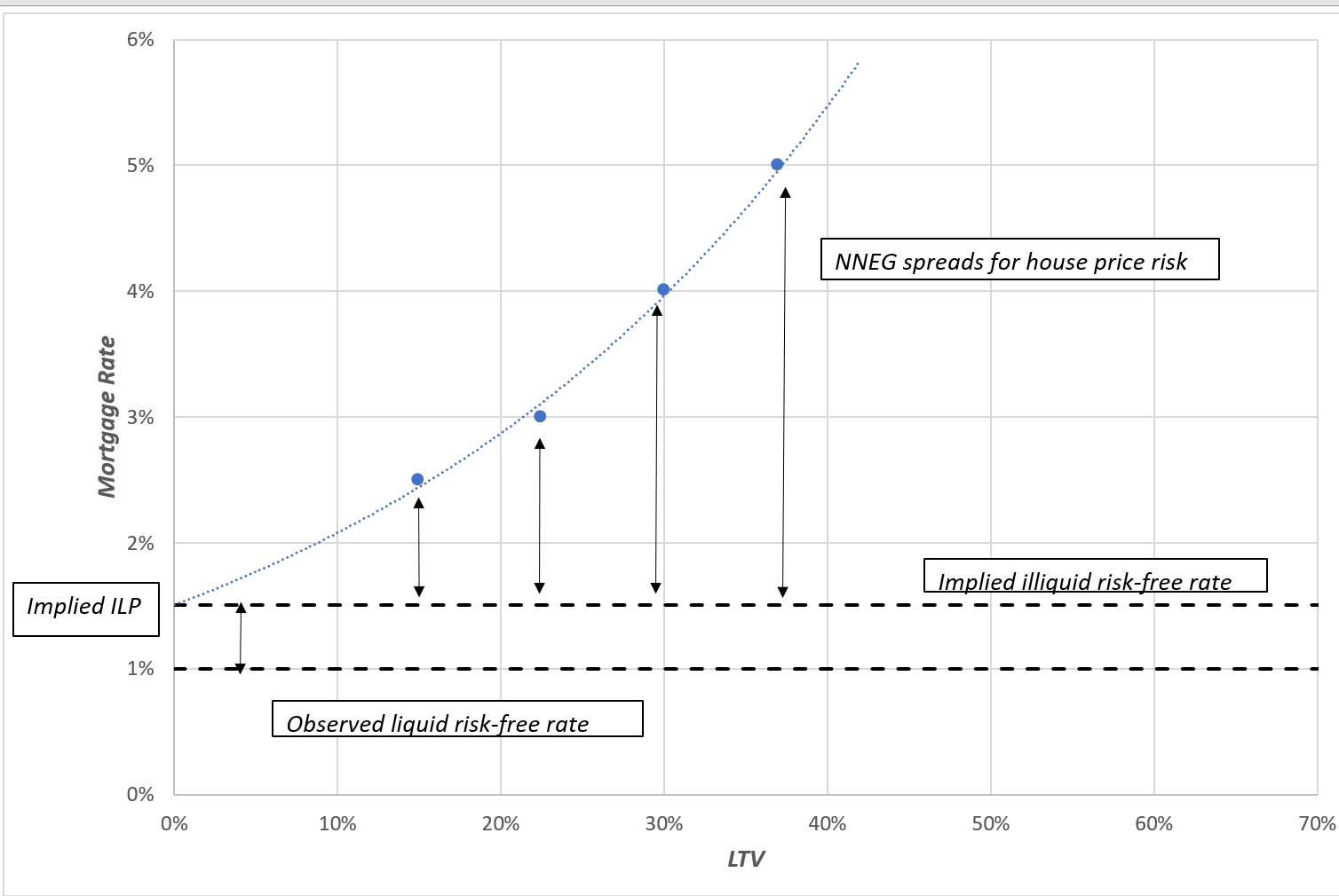
Let’s consider a hypothetical example (I use a hypothetical example because origination equity release mortgage rates and their variation by LTV are not fully publicly disclosed; but it is normal practice for mortgage writers to use origination prices for a range of LTVs in the calibration of their mortgage valuation basis). You may recall my July 2020 valuation methodology research paper[1] in which example valuation model calibrations were developed using a number of hypothetical origination ERM mortgage rates that spanned a range of borrower ages, with two different LTV levels per age. For our current purposes, let’s suppose we can observe a few more mortgage rates at various LTVs for each given age – instead of two LTVs per age, we suppose there are four (a further two mortgages rates at other LTV levels in addition to the two specified in the paper). Again, this is not an unusually rich set of ERM origination prices to work with, in the context of typical ERM valuation practice. The chart below plots the four LTVs and origination mortgage rates that are associated with borrowers aged 60. It also plots a simple exponential trendline that is fitted through these four prices[2].
Exhibit 1: De-composition of observed (hypothetical) origination mortgage rates (borrower age 60)
The extrapolation of the trendline to 0% LTV provides an estimate of the illiquid risk-free rate – in this example, the trendline crosses the x-axis at 1.51%. We know the liquid risk-free rate – in this exercise it has been assumed to be 1.0%. And, so, we have obtained an estimate of the mortgage-implied illiquidity premium of 0.51%. Let’s not be actuarially spurious, we’ll call it 0.5%.
We could repeat this exercise for mortgage rates of different borrower ages. Each would likely provide a slightly different mortgage-implied illiquidity premium. Such variation would reflect the limitations and estimation errors of extrapolation. My (educated) guess is that these variations in the estimate of the mortgage-implied illiquidity premium would not be very material.
Of course, like any extrapolation, this process is fallible and imprecise. You might question why an exponential function is the ‘right’ functional form for this extrapolation. Perhaps we should use a valuation model to justify a particular form of extrapolation function. That might possibly be quite useful. But rather than make the illiquidity premium estimate a function of a particular structure of valuation model, perhaps we can appeal to a bit of common sense here. In this example, there are some things we can be confident of, irrespective of the choice of extrapolation function. For example, the mortgage-implied illiquidity premium in this example is not 3%. Nor is it not 4%. If the mortgage writer is prepared to write a risky mortgage at a rate of 2.5%, and the liquid risk-free rate is 1.0%, the illiquidity premium logically cannot be bigger than 1.5% (even if this mortgage is considered completely risk-free and there are no costs associated with writing the mortgage). In my view, this simple extrapolation process from observed origination prices delivers a reasonable assumption for the mortgage illiquidity premium – 0.5% in this example – and does so in a very transparent and logical way. This assumption can then be employed consistently in the valuation basis for all mortgages in the in-force portfolio (and indeed in the valuation of securitisations, if we assume the securitisations are also similarly illiquid).
A few final thoughts on illiquidity premium, fair valuation and the Matching Adjustment
The above analysis has argued that, as mortgages of varying LTVs have essentially the same degree of illiquidity, they ought to be valued assuming the same illiquidity premium. But it might be argued that the illiquidity premium in high-LTV mortgages really is bigger than the illiquidity premium in the lower LTV mortgages. That is, if a liquid version of these assets were created, the effect of this liquidity would be to increase the high-LTV mortgage values by more than it would increase the value of the lower LTV mortgages. This assertion, being based on a hypothetical and unobservable scenario, is impossible to disprove. But my guess would be that what an actuary really means when they say a high-LTV mortgage has a higher illiquidity premium than a low-LTV mortgage is that it offers a more attractive expected return – it is an expression of a view of the relative cheapness / dearness of the assets. It may well be a perfectly reasonable view; I can offer no useful insight into that. But my point in response would be that such a view has no natural role to play in a fair valuation process – fair valuation merely requires the valuation to be consistent with a set of observed prices; whether we believe those observed prices to be cheap or dear is simply neither here nor there.
Whether such a view of relative cheapness / dearness is relevant to the Matching Adjustment is a more open question. There would seem to be little doubt that general (i.e. beyond ERM) Matching Adjustment practice has moved beyond its original rationale of allowing for the capitalisation of illiquidity premia and has also allowed for capitalisation of at least a portion of the risk premium embedded in the pricing of credit-risky assets. In such circumstances, the assessment of the expected return of the assets is a required input, and this can bring views of the relative cheapness / dearness of the assets into play. Whether or not this is really a desirable feature of a regulatory solvency system is an interesting and important question, but this is certainly not a question specific only to equity release mortgages.
Postscript
EIOPA’s Opinion on the 2020 Review of Solvency II was published during the writing of this note. Its section on Matching Adjustment is potentially relevant to above discussion, especially Section 2.17: “where the underlying assets include financial guarantees, those guarantees do not increase the Matching Adjustment”. This sounds like an argument for restricting the Matching Adjustment discount rate, in the above terminology, to the illiquid risk-free interest rate (i.e. the liquid risk-free interest rate plus the estimated illiquidity premium). This would mean, in the case of ERMs, that the MA’s Fundamental Spread would make full allowance for the market-consistent cost of NNEG risk, rather than only deducting expected losses and leaving some risk premium in the MA discount rate. These EIOPA words also appear consistent with PRA SS3/17’s Section 3.20: “Compensation for these NNEG risks should not lead to MA benefit”. These statements can only increase the usefulness and importance of a transparent and objective approach to estimating the illiquidity premium applicable in mortgage valuations (and hence the component of compensation that is not arising from NNEG risks or other financial guarantees).
[1] See A Valuation, Capital and Matching Adjustment Methodology for Equity Release Mortgages | Craig Turnbull FIA
[2] The trend line for the age 60 mortgage rate is 0.0151.exp(3.2194 x LTV).
[1] See my March 2020 note for fuller technical discussion of the effect of illiquidity on derivative valuations: Notes on Derivative Valuation and Illiquid Assets | Craig Turnbull FIA
[1] See my May 2020 article on prepayment risk for a fuller technical discussion of this topic: Prepayment Risk and Equity Release Mortgages | Craig Turnbull FIA
No Comments