
17 Jul 2019 On the Actuarial Treatment of Equity Release Mortgages: Part Two
My article of 13th June surveyed some of the recent research on the actuarial treatment of equity release mortgages (ERMs) and discussed approaches that can be taken to fair valuation and the assessment of capital requirements. This article considers how the approaches that were identified as reasonable in that article compare with current actuarial practice.
Discerning current actuarial practice on the treatment of ERMs is not completely straightforward. The methods used by firms in their ERM valuations and capital assessments are not fully in the public domain. Firms’ Solvency Capital Requirement (SCR) Internal Models are privately submitted to the PRA. Firms are not obliged to disclose the SCR they are holding in respect of specific asset classes such as ERMs. Firms do provide some description of their fair value methodology in Annual Reports and Accounts and in Solvency and Financial Condition Reports, but these descriptions are generally incomplete. Moreover, terminology may be used differently by different firms (and researchers), and so the need for some interpretation is inevitable.
Firms do, however, disclose some of their key valuation assumptions and some publish some key valuation sensitivity results. We can use the limited public disclosure of valuation methods and assumptions to try to join the dots on how valuations have been implemented. And the disclosed sensitivity test results can be used to attempt to corroborate our interpretation. This is a messy and fallible process undertaken from a semi-informed vantage point. It inevitably involves some art as well as science. Nevertheless, it may still be possible to obtain some significant insights into current actuarial practice and how it compares with the approaches suggested in the 13th June article.
A Case Study: Just Group plc’s end-2018 ERM valuation approach
As a focused UK insurance group with a significant portion of its investments allocated to ERMs, Just Group may provide a good illustrative case study of current actuarial practice. Just Group has also provided more disclosure of ERM valuation assumptions and ERM valuation sensitivities than some of the other major UK insurance firms that materially invest in ERMs. For these reasons only, we will focus on Just Group’s valuation approach in our illustrative case study. However, to provide further context to UK practices, we will also consider some of Legal & General Group’s (L&G’s) statements on its end-2018 ERM valuation methods.
In its end-2018 Annual Report and Accounts, Just Group valued its ERMs (Lifetime Mortgages in their preferred parlance) at £7.1915bn (representing more than one-third of its total investment portfolio of £19.252bn). The Annual Report states that Just Group values its ERM No-Negative Equity Guarantees (NNEGs) using ‘a variant of the Black-Scholes model’ (p. 123). The Annual Report also discloses that the following parameters were used in the valuation: house price volatility of 13% (p. 27); deferment rate of +0.3% (p. 27); house price growth of 3.8% (p. 126).
L&G’s end-2018 Annual Report contains fewer specifics about its ERM valuation methods. The Report notes that the ERM valuation depends on a property price volatility assumption (p. 108), but it does not disclose what assumption has been used. L&G do, however, specify that they have used a long-term house price growth assumption of RPI + 0.5% (p. 149), which suggests a very similar house price growth assumption to that used by Just Group.
At first glance, the Just Group disclosures might suggest it is very straightforward to understand exactly how Just Group has valued its ERMs: a Black-Scholes formula with stated volatility and deferment rate (i.e. income yield) assumptions has been used to value the NNEG; the SII yield curve is prescribed and so was presumably used as the risk-free rate in the Black-Scholes valuation and in the valuation of the risk-free component of the ERM cashflow stream. (Further complications will follow around the Matching Adjustment treatment and the valuation of the tranches of any ERM securitisations, but these come after the basic valuation of the ERMs and are beyond the scope of this article.)
Just Group’s (and L&G’s) valuation assumption disclosures, however, raise an interesting question: why is there a stated assumption about house price growth? The Black-Scholes NNEG valuation does not make any assumption about house price growth. Indeed, as noted in the previous article, it is one of the basic insights of option pricing theory that an option value does not depend on the assumed growth rate of the underlying asset.
Technically, the underlying asset growth rate assumption has two offsetting impacts on the option valuation: it changes the distribution of the projected cashflow and, therefore, its expected value; and it changes the discount function that is applied to the projected cashflow. Option pricing theory shows that these two effects cancel out. We can assume the house price growth is +1000%, the risk-free rate, +3.8%, -3.8% or -1000% and we will still get the same option value (if we do the sums correctly[1]). This is why the expected return of the underlying asset does not appear in the Black-Scholes formula.
But Just Group state they have assumed house price growth of 3.8% and L&G state a very similar assumption. This suggests their valuation methodologies are sensitive to this assumption. The ‘variant’ dimension of Just Group’s stated Black-Scholes NNEG valuation method must be referring to the use of the house price growth assumption, but no further guidance is provided on what variation has been made.
There is another aspect of Just Group’s disclosed valuation assumptions that we need to consider further. The example calculations of my previous article suggested that using a volatility of 13% and a deferment rate of +0.3% in a Black-Scholes valuation would tend to produce very small values for the NNEG. This, in turn, would imply day-1 values for the ERM that are much higher than the amount loaned. Briefly returning to the example of the 13th June article, these parameter choices produce a NNEG valuation of 0.054 (whereas our suggested methodology produced a valuation of 0.200); and an ERM valuation of 0.50. That is, a loan of 0.30 generates a day-1 fair value of 0.50. It would be extremely surprising if firms were really producing day-1 asset values in their Solvency II balance sheet that were two-thirds greater than the amount loaned. This is surely not what is happening.
To recap, we have made two observations: a standard implementation of Black-Scholes with Just Group’s stated volatility and deferment rate parameters would produce a day-1 ERM valuation well in excess of the loan amount; Just Group (and L&G) have used a house price growth assumption in their ERM valuations, but it is not clear how. Is there a simple way of explaining and reconciling these two observations? I think there probably is. A house price growth assumption of 3.8% and a deferment rate (income yield) of 0.3% together imply a property total return assumption of 4.1%. It seems plausible that Just Group have used this property total return assumption of 4.1% as the risk-free interest rate parameter in their Black-Scholes NNEG valuation, and have also used that value, or a very similar value, as the discount rate in the valuation of the risk-free cashflow component of the ERMs.
This interpretation is consistent with L&G’s description of their valuation methodology. L&G’s Annual Report (p. 149) states that their equity release mortgages have been “valued using a discounted cashflow model by projecting best-estimate net proceeds and discounting using rates inferred from current LTM [Lifetime mortgage] pricing.” The term “best-estimate net proceeds” implies that the expected cashflow of the NNEG has been assessed using the stated house price growth assumption together with some (undisclosed) property volatility assumption. Current roll-up rates of equity release mortgages are typically 4%-4.5% (see 13th June article), suggesting an assumption of this order this has been used as the discount rate “inferred from current LTM pricing”. So L&G’s disclosed description of their valuation method appears quite consistent with the above interpretation of Just Group’s stated method.
In our simple example of 13th June, a risk-free rate of 1.5%, with a house price volatility of 16% and deferment rate of 3.0% produced an ERM value of 0.351. This was derived as the risk-free cashflow component (0.551) less the NNEG (0.200). Now suppose we value the same example ERM with the assumptions suggested by Just Group’s disclosures: that is, a risk-free rate of 4.1%, a house price volatility of 13% and a deferment rate of 0.3%. In this case, the risk-free component has a value of 0.293 (= 0.300 x 1.04025/1.04125) and the NNEG has a value of 0.005 (obtained from the Black-Scholes formula). The ERM is therefore valued at 0.288 (and recall the amount loaned was 0.300).
This is, of course, based only on a single highly illustrative example, but it suggests the Just Group valuation basis, interpreted in this way, could produce a very sensible day-1 ERM asset valuation. Indeed, it might even suggest that the ERM valuation calibration has been parameterised to produce a day-1 valuation equal to the initial loan size (i.e. no day-1 gain). (Bear in mind the parameterisation of the example ERM has not considered Just Group’s actual roll-up rate basis or any other feature of its pricing approach, so the proximity of the ERM valuation with the loan amount is arguably surprisingly close. For example, if we changed the assumed roll-up rate of the example ERM from 4.00% to 4.17%, we would obtain a day-1 ERM valuation of exactly 0.300 with our interpretation of the Just Group valuation methodology.)
We can gain some further corroboration of this tentative interpretation of Just Group’s valuation method by considering their published ERM valuation sensitivities. In particular, we can compare these published sensitivities with the fair value sensitivities produced when our interpretation of Just Group’s valuation method is applied to our single example ERM of the previous article. Of course, we would expect significant differences to arise because the single example policy is only that. It has not been parameterised to represent Just Group’s ERM book in any way, and therefore cannot be expected to behave in exactly the same way. But if we see sensitivities of a similar order of magnitude, that may be supportive of our tentative interpretation.
The comparison of fair value sensitivities produced in Just Group’s end-’18 annual report and those produced our single example mortgage with our interpretation of the Just calibration can be summarised as follows:
- A +0.5% increase in deferment rate resulted in a 1.1% decrease in ERM fair value in the Just Group annual report; and a 0.8% decrease for our example mortgage;
- A 10% property price fall resulted in a 1.4% decrease un ERM fair value in the Just Group annual report; and a 0.7% decrease for our example mortgage;
- A 1% increase in property volatility resulted in a 0.7% decrease in ERM fair value according to both the Just Group annual report and our example mortgage.
The deferment rate and property volatility sensitivities are quite similar. There is a more material difference in the property price fall sensitivities. Just Group’s higher reported sensitivity to property price falls is consistent with their ERM portfolio having a spread of mortgages that includes some mortgages with higher Loan-To-Value levels (the NNEGs of such policies will have larger deltas). The comparison of these sensitivities suggests we are on the right track.
Similar day-1 ERM valuations; very different NNEG valuations and credit risk estimates
The above discussion suggests we can tentatively conclude that the valuation methods and assumptions proposed in the 13th June article can produce a similar day-1 ERM asset valuation to the methods and assumptions described by Just Group. Furthermore, these day-1 ERM valuations are at intuitive levels consistent with the starting loan amount. Might we therefore conclude that this is the end of the matter?
Well, before we move on to something more interesting, it is worth emphasising that these two valuation calibrations are very different. They may be able to produce very similar valuations on day-1, but that does not mean they will give similar results on day-1000 or day-10,000. In particular, although the two valuation approaches can produce similar initial ERM valuations, in doing so they produce radically different NNEG valuations.
These differences in NNEG valuation reflect the substantial differences in the scale of the house price risk that are implied by the two calibrations. The Just Group parameterisation suggests the ERM has very little house price risk on day-1, whereas the parameterisation suggested in the 13th June article implies the house price risk is quite material. This has consequences for the sensitivity of the day-1 fair value to changes in house prices (and other risk factors). The chart below shows how the fair value sensitivities of our single example ERM compare when using our interpretation of the Just Group end-’18 valuation method and the valuation calibration of the 13th June article.
Exhibit 1: Fair Value Sensitivities
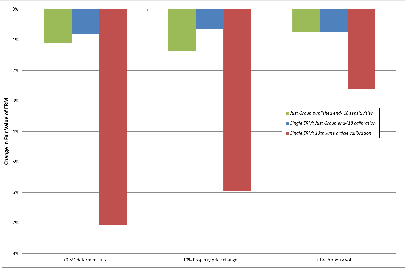
So, whilst the two calibrations may produce similar day-1 valuations for our single example ERM, they produce very different risk sensitivities. If the measurement of the ERM’s Solvency Capital Requirement (SCR) is aligned to the 1-year VaR of the ERM fair value, this implies the assessed SCR will be materially different in the two cases. You may recall from the 13th June article that the calibration used there suggested an SCR of 30% or so for the single example ERM (prior to MA and any re-structuring). By the same logic, the fair value sensitivities produced by the end-’18 Just Group calibration would be consistent with an SCR of around 7% to 8% (again prior to any MA benefit and re-structuring). Roughly speaking, these SCR assessments differ by a factor of 4 or 5.
Illiquidity Premium
We might wonder why it is thought reasonable to assume a 4.1% risk-free interest rate in a Solvency II balance sheet asset valuation at a time when the SII long-term risk-free rate was approximately 1.5%. One way to rationalise this would be to call the c. 260 basis point difference an ERM illiquidity premium. Again, the disclosures in L&G’s end-2018 Annual Report also paint a consistent picture. In the description of their ERM valuations they note that “the inferred liquidity premiums for the majority of the portfolio range between 100 and 350 basis points”.
The idea of an illiquidity premium – that illiquid assets are priced to yield more than risk-equivalent liquid assets as compensation for illiquidity – is central to the significant rotation from public to private credit market allocations that is currently underway in UK annuity asset portfolios (and elsewhere). In general, the illiquidity premium implied by market prices is quite difficult to measure: there may be no readily observable market price for an illiquid asset; it may be difficult to find two truly risk-equivalent assets from which to infer the illiquidity premium; and asset liquidity is not a binary state, so, when trying to estimate the illiquidity premium, the question arises of what degree of illiquidity is associated with the ‘illiquid’ asset (and the liquid one, for that matter).
To take a simple example, we can note that UK government-guaranteed Network Rail bonds tend to offer a yield pick-up of around 20 basis points in excess of UK gilts (Eumaeus blog, 21st June 2019). This suggests the illiquidity premium offered by the Network Rail bonds is, at most, 20 basis points (if we view the Network Rail bonds as more credit-risky than UK gilts, then part of the 20 basis points must be a credit risk premium and the illiquidity premium must therefore be less than 20 basis points). Does this observation allow us to infer that the market’s illiquidity premium is 20 basis points? It is certainly a useful reference point, but the difficulty with this inference is that asset liquidity varies by degree across assets. It might be argued that an equity release mortgage is materially less liquid than the Network Rail bond, and, hence, should command a substantially greater illiquidity premium. There is a qualitative logic to that argument, but it is difficult to transform it into reliable numbers. How much less liquid is the ERM relative to the Network Rail bond? And how much greater should its illiquidity premium therefore be? No easy answers are forthcoming (from me, anyway).
For reasons such as above, the direct estimation of the illiquidity premium by comparison of liquid and illiquid asset prices is rarely made. It is more typical to infer the illiquidity premium on a private credit-risky asset indirectly by making an assessment of the asset’s credit risk, and the spread (expected default loss and credit risk premium) required to compensate for that risk. The illiquidity premium is then defined as the excess of the asset’s gross spread over the assessed credit-required spread. This clearly places the onus on assessing the ‘correct’ credit spread for the private credit asset (by which we mean the spread that the credit-risky asset would trade at if it was very liquid). Private credit assets often have credit risk profiles that are distinctly different to public credit assets. The risks of private credit assets may be more heterogeneous and subject to less public scrutiny and standardisation – for example, many private credit assets will not have a public credit rating from the established rating agencies.
In such circumstances, there may be a danger that firms mistakenly arrive at unduly optimistic assessments of an asset’s credit risk and explain it by reference to the existence of a large illiquidity premium. This potential danger arguably exists in the treatment of any credit asset class. But it has greater potential for error when there is significant uncertainty around the size of the illiquidity premium that the asset should command; and where the credit risk of the asset is not independently assessed through publically-recognised methods.
Returning one last time to our single illustrative ERM, we see that this de-composition of spread between credit risk and illiquidity premium is very pronounced under our interpretation of the Just Group method. The NNEG fair valuation produced by this calibration implies an ERM credit spread of less than 10 basis points (which sits alongside an illiquidity premium of some 260 basis points). L&G’s more limited disclosures suggest an approach consistent with Just Group’s. By contrast, you may recall from our 13th June note that the calibration suggested there produced a credit spread of 185 basis points as compensation for the NNEG risk in the example ERM.
In Summary
This article has tried to shed some light on how current actuarial practices on the treatment of ERMs compare with those suggested in my LinkedIn article of 13th June. Based on Just Group’s public disclosures of end-2018 valuation assumptions and valuation sensitivities (and, to a lesser degree, the more limited disclosures of L&G), we tentatively identified the type of approach currently being used to value ERMs. We found the approach could produce day-1 ERM fair values that were consistent with the initial loan amount. However, the approach produces ERM fair values with materially less sensitivity to key risk factors such as house price falls. If the SCR methodology is aligned to fair value sensitivities, this approach would therefore produce a materially lower SCR than that produced by the calibration suggested in the 13th June article. These current valuation approaches imply that the vast majority of the spread earned by an ERM is an illiquidity premium rather than a spread to compensate for NNEG risk. The ERM credit spread implied by the Just Group calibration is much smaller than the ERM credit spread implied by the 13th June article calibration.
This article has not considered the substantial further complications that arise in insurance firm’s actuarial treatment of ERMs. In particular, we have not considered the implications of the re-structuring of the ERMs, the application of the Matching Adjustment to the senior tranche of those re-structures, or the impact of SII transitional measures. We have only been concerned with the fair valuation of the underlying equity release mortgage assets on the SII balance sheet, and the implications of the fair value behaviour for a consistently assessed SCR.
The analysis that has been undertaken here is entirely based on very limited public information and should therefore be viewed as fallible and tentative. It certainly should not be regarded as quantitatively reliable. The qualitative conclusions, however, appear quite intuitive in the context of the ongoing industry debate about the actuarial treatment of equity release mortgages.
Disclaimer
This article is written in a personal professional capacity as a Fellow of the Institute and Faculty of Actuaries, and is intended solely as a discussion of technical actuarial methods.
[1] See, for example, Asset Pricing, John Cochrane (2005); Modern Valuation Techniques, Jarvis, Southall and Varnell (2001).
No Comments