22 Aug 2019 On the Actuarial Treatment of Equity Release Mortgages: Part Three

The vast majority of UK insurers’ investments in equity release mortgages are held in a form of structured vehicle. My previous two notes on the actuarial treatment of ERMs have focused on treatment of the underlying mortgages, and have not considered the nature and effect of these re-structuring efforts. This note considers how the previous discussions on the valuation and assessment of risk and capital requirements of ERMs can be extended and applied to the valuation and assessment of the risk and capital requirements of the types of ERM structured solutions that are currently being used by most, if not all, of the major ERM-investing UK insurance firms.
We (again) defer explicit consideration of the impact of Solvency II’s Matching Adjustment (MA) to a later discussion. An appropriate MA treatment can only be developed and evaluated after the fair valuation and risk and capital requirements of these assets have been assessed in the absence of the MA.

Re-structuring the ERMs – the basic idea

The basic idea is as follows. An insurer’s portfolio of equity release mortgages is placed inside a Special Purpose Vehicle (SPV). In the simplest setting, the capital structure of the SPV will have two components: a senior, or debt, component (or tranche, in SPV jargon), which promises to pay a specified set of fixed cashflows until a specified maturity date; and a junior, or equity, component (tranche), that has a claim on the residual assets of the SPV once the debtholder has been paid in full. If the assets of the SPV are not sufficient to pay the senior tranche in full, the holder of the senior tranche receives all the assets in the SPV and the holder of the equity tranche receives nothing.
As far as I am aware, in all cases to date, UK insurance firms have retained full ownership of the entire capital structure of these ERM SPVs, and all the assets inside the SPV were fully-owned by the insurer prior to the re-structuring. The insurance firm’s economic exposure to its ERM portfolio is therefore exactly the same as it was before the portfolio was placed inside the SPV. The use of the SPV is, to date, simply a cosmetic re-presentation of the assets in a way that makes a portion of these assets eligible for use in backing Matching Adjustment (MA) liabilities. In doing so, the re-structuring thereby potentially allows the insurance firm to access all the benefits that arise under the MA (such as a reduction in liability valuation, a reduction in solvency capital requirement, and faster profit recognition).

Valuing the tranches of the SPV

In keeping with the methods of the previous ERM articles, we will develop insight into the nature of this problem through the use of a simple case study. In fact, we will use the same example equity release mortgage as the one discussed in the previous two ERM articles (Part One and Part Two). To re-cap, we assumed a risk-free interest rate of 1.5%; a property deferment rate of 3.0%; house market index volatility of 12%; house-specific volatility of 11%; and the mortgage was assumed to have an initial Loan-To-Value of 30%; a mortgage roll-up rate of 4.0% and a term of 25 years.

The aggregation of the house market index volatility of 12% with the (uncorrelated) house-specific volatility of 11% produces a total house price volatility of 16% pa. To further re-cap, this mortgage has a promised payment at maturity (25 years) of 0.800. In the Part One article, we found that the present value of the certain component of the mortgage is 0.55; and the no-negative equity guarantee has a value of 0.200, resulting in an overall equity release mortgage value of 0.35. The fair value implies a gross redemption yield on the mortgage asset of 3.35%, which in turn implies a credit spread of 185 basis points over the assumed risk-free rate.

The good news is that we do not need to make any further valuation assumptions in order to value any tranche of an SPV of a portfolio of the above ERMs. Suppose we write mortgages with the above terms on 1000 different houses. The value of the 1000 mortgages is clearly 350 (i.e. 0.35 x 1000). Let’s further suppose that we put these 1000 mortgages into an SPV that issues a senior or debt tranche and a junior or equity tranche.

The above economic, property and mortgage assumptions uniquely define a value for any tranche of this vehicle. Given these assumptions, valuing the tranches is in fact very straightforward: they are well-defined forms of contingent claim. To my (limited) knowledge, a closed-form solution for the valuation of the tranches according to the above modelling assumptions is not readily to hand, but the valuations can be implemented using standard Monte-Carlo simulation techniques (like those used by UK life actuaries for the last 15 years or more in areas such as the fair valuation of with-profit guarantees).

With the portfolio of 1000 mortgages, the total promised cashflow of the SPV amounts to 800 (= 0.800 x 1000). Of course, to receive the full promised 800, every single one of the 1000 mortgages would need to be re-paid in full, and this will be a very rare occurrence (we will have a more sustained discussion of the probability distribution of the pay-outs in a forthcoming Part Four article).

As a simple starter for ten, let’s consider the valuation of the SPV tranches when the debt tranche promises to make a single payment of 500 at the end of the 25-year term of the mortgages (in SPV jargon, this amount is called the attachment point of the capital structure). If we plug this 500 attachment point into the simulation valuation model with the parameters of Exhibit 1, we obtain a fair value of 297 for the debt tranche and 53 for the equity tranche (and so the debt-to-asset ratio of the SPV is 85%). Note the two values add up to 350, the total value of the underlying ERMs. It is a simple no-arbitrage condition that the values of the capital structure of the SPV must sum in total to the value of the underlying asset portfolio.

The debt tranche of the SPV therefore has a gross redemption yield of 2.11% (= (500 / 297)^(1 / 25)-1). And its credit spread is therefore 0.61% (= 2.11% – 1.50%).

It may seem a bit incongruous to talk of promised cashflows and gross redemption yields on an equity asset, but this clearly isn’t an equity asset in the usual sense – it is still a slice of the cashflows from a set of fixed interest loans. The promised equity cashflow is 800 – 500 = 300. It therefore has a gross redemption yield of 7.18% (= (300 / 53)^(1 / 25)-1) and a credit spread of 5.68% (= 7.18% – 1.50%).

To re-cap so far: we have started with a pool of 1000 assets with a total starting value of 350, a gross yield of 3.35% and credit spread of 1.85%; and we have re-structured this asset portfolio into two assets, one that is less risky, lower-yielding and valued at 297, and another that is riskier and higher-yielding and valued at 53.

We can re-run the above numbers for any attachment point for the SPV tranches. Exhibits 1 and 2 show the fair values and credit spreads produced for the full range of possible attachment points for our example SPV.

Exhibit 1: Fair values of equity and debt tranches as a function of attachment point

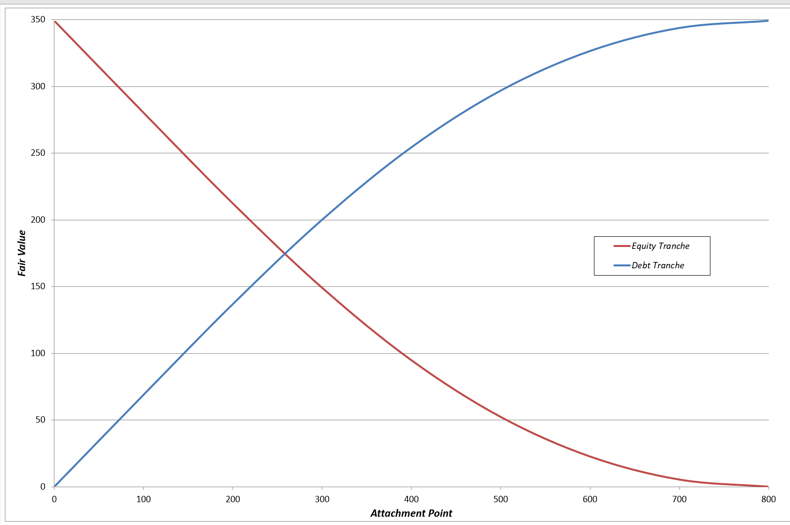
Exhibit 2: Credit spreads of equity and debt tranches as a function of attachment point

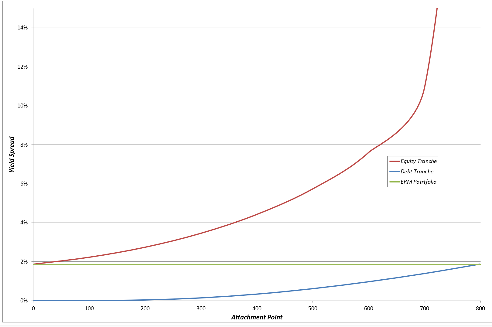
With an attachment point of 0, there is effectively no re-structuring, and the equity tranche simply represents the total portfolio of ERM assets. The equity tranche in this case therefore has a spread of 1.85% (i.e. the spread of the underlying mortgages). At the other end of the chart, with an attachment point of 800, now it is the debt tranche that represents the total ERM assets, and it therefore has a spread of 1.85%. As we increase the attachment point from 0, the value of the debt increases, the value of the equity decreases, and the yields of both equity and debt increases. The total value of the underlying asset portfolio (350) and its yield (3.35%) and spread (1.85%) are unaffected by the choice of attachment point.

SPV Tranche Valuations: Caveats and Complications

The key conclusion of the above analysis is that, once settled on a valuation methodology for the underlying mortgages, the consistent valuation of the SPV tranches is relatively straightforward. There are a couple of caveats that should be added to this conclusion, which are discussed below.

The valuation of the SPV tranches may be sensitive to assumptions that are not relevant when valuing the underlying mortgages. In particular, the valuation of a tranche of the SPV is a function of the form of co-dependency that is assumed between the underlying mortgages. This assumption has no bearing on the value of the mortgages themselves.

In our model, the co-dependency between the mortgages is determined by the volatility structure we have assumed for the underlying house prices. And the volatility structure we have used is a simple one: there is a single market or index factor that all houses are assumed to have the same exposure to; and every house is then assumed to have an equally-sized idiosyncratic source of risk that is independent of the house index and independent of the idiosyncratic risk of every other house. And both the index and idiosyncratic sources of risk are assumed to have normal distributions. These assumptions imply that the house prices have a Gaussian joint dependency structure, with a correlation of +0.54 between the price changes of any two houses and a correlation of +0.74 between the price changes of any house and the market index[1]. This provides a reasonable starting point, but the dependency structure could arguably be more complex than the Gaussian assumption, and the tranche valuations could be particularly sensitive to this assumption for some levels of attachment point.

Secondly, as noted in the Part One and Part Two articles, there is currently relatively little industry consensus on the valuation assumptions that ought to be used in the fair valuation of the underlying mortgages. Different valuation assumptions for the mortgages may imply different valuation results for the SPV tranches.

Suppose, in the spirit of the Part Two article, that a fair valuation method is used that produces the same fair values for the underlying mortgages as the valuation basis used above, but does so by assuming that most of the mortgage spread is an illiquidity premium rather than a credit risk premium. That is, a lower volatility and lower deferment rate is assumed in the ERM valuation basis, together with a higher risk-free interest rate that results in the same mortgage fair value as the Part One article basis.

In such a case, the tranche fair values at attachment points 0 and 800 are unaffected, as these are generated by basic no-arbitrage conditions that are not sensitive to changes in these assumptions (when the fair values of the underlying mortgages are unchanged). Similarly, for any and all attachment points, the values of the equity and debt tranches still must sum to the total fair value of the underlying mortgages. And the credit spreads of the tranches will still be monotonically increasing functions of the attachment point.

But the alternative ERM valuation basis implies there is much less credit risk in the SPV (recall how the Just Group assumptions implied our underlying example ERMs’ spread to compensate for credit risk was around 10 basis points instead of the 185 basis points implied by the Part One valuation basis). And this means that the debt of the SPV has exceedingly little credit risk at attachment points of less than 600 or so. At these levels, the debt tranche is essentially risk-free and has zero spread for credit risk – all of the spread therefore has to be attributed to an illiquidity premium effect. At an attachment point of 600, the debt tranche has a 1bp credit spread, which eventually rises to the 10 or so bps of the spread of the underlying ERMs as the attachment point reaches 800.

Exhibit 3 compares the fair values produced for the two tranches according to the two alternative valuation bases for the underlying ERMs.

Exhibit 3: Fair values of equity and debt tranches as a function of attachment point (with alternative ERM valuation bases)

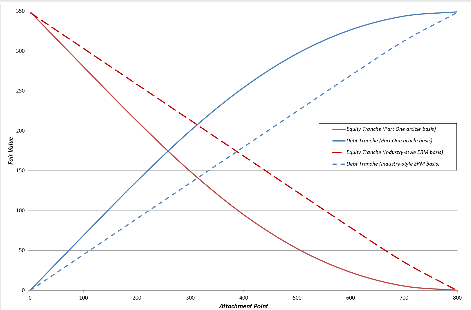
The chart shows that the industry-style ERM valuation basis results in lower valuations for the SPV’s debt tranche and a correspondingly higher valuation for the equity tranche. It might seem peculiar that the debt tranche has been reduced by the shift to a valuation basis that assumes the underlying assets are less risky – after all, the debt is basically short a put option on the end-period portfolio value. This effect is due to the significant illiquidity premium that is embedded in the interest rate basis of this valuation approach. For example, with an attachment point of 500, the industry-style valuation of the debt tranche is 225. This implies a yield of 3.25%, and hence a spread of 1.75%. But only 1 basis point of that spread can be attributed to the credit risk produced by this valuation basis. The remaining 174 basis points of spread is illiquidity premium.

The equity tranche valuation represents the other side of this coin. The lower debt tranche valuation, which is very useful for generating MA-efficient yield, must result in a correspondingly higher equity tranche valuation. At the attachment point of 500, which might be tentatively viewed as producing a typical level of debt-to-asset ratio for these types of ERM structured vehicles, the industry-style method has produced an equity tranche valuation that is more than twice as big as the value produced by the Part One valuation basis. This may be one factor that makes it difficult for insurance firms to find potential buyers for the equity tranches of these ERM SPVs – their valuation method may produce equity tranche valuations that are higher than might be implied by a more economically-intuitive ERM valuation basis.

Assessing the Solvency Capital Requirements of the SPV Tranches

The Part One article discussed a fair value-based approach to assessing the SCR of an individual ERM. This same approach can be directly applied to the SPV tranches. In Part One, an individual ERM was re-valued under stress very easily as there was a closed-form valuation formula for the ERM (that used the Black-Scholes formula for the NNEG put option). For the SPV tranches, the lack of a closed-form valuation solution means we will re-value using the Monte-Carlo simulation valuation engine.

The following stress test results for the tranche valuations are obtained when the attachment point of 500 is used:

• In the base case, the 1000 ERMs have a fair value of 350 and their NNEGs have a value of 200. The SPV’s debt tranche is valued at 297 and the equity tranche is 53.
• In the 40% property price stress test, the 1000 ERMs have a fair value of 250 and their NNEGs have a value of 300. The SPV’s debt tranche is valued at 232 and the equity tranche is 18.
• In the 16% to 20% volatility stress test, the 1000 ERMs have a fair value of 315 and their NNEGs have a value of 235. The SPV’s debt tranche is valued at 265 and the equity tranche is 50.

The results for the ERM and NNEG fair values are the same as those produced in the Part One article. We found there that the 40% house price fall implied a 29% capital requirement for the ERM (i.e. 1 – 250/350). We can now also see that if we put 1000 of these mortgages into an SPV with an attachment point of 500, we assess a property stress SCR of 22% for the debt tranche and 66% for the equity tranche. Similarly, we found in the Part One article that the volatility stress resulted in a 10% capital requirement for the ERMs (i.e. 1 – 315/350). We can now see that the volatility stress SCR for the debt and equity tranches of the SPV are 11% and 6% respectively.

The house price stress results are quite intuitive: the equity tranche is riskier than the debt tranche and hence attracts a higher SCR. It may be much less obvious why the equity tranche has a lower sensitivity to volatility increases than the debt tranche, and why the debt tranche has a higher volatility sensitivity than the underlying ERMs. But there is a sensible explanation.

The reason is that two partially off-setting effects impact on the value of the equity tranche when house price volatility increases. In a nutshell, the equity tranche is a long call option on a portfolio that is short put options. On the one hand, the volatility stress results in the underlying ERMs being reduced in value (from 350 to 315), because of the increase in the NNEGs that arises when volatility increases. This fall in the underlying asset value has the effect of reducing the value of the equity tranche. But on the other hand, because the equity tranche is a call option on the ERM portfolio, an increase in the volatility of the ERM portfolio has the effect of increasing the value of the equity tranche. These two effects move in opposite directions.

Meanwhile, the debt tranche can be viewed as a risk-free asset less a put on the ERM portfolio value. The debt tranche is therefore short a put option on a portfolio that is short put options. It therefore suffers a ‘double-whammy’ valuation hit when house price volatility increases: the underlying asset value falls and the underlying asset becomes riskier. Both of these have a negative impact on the value of the debt tranche. Consequently, the debt tranche has a volatility SCR that is greater than that of the underlying ERMs.

There are some subtleties to consider when specifying each of these stress tests for the purposes of re-valuing the SPV tranches. In particular, when specifying the volatility stress, we need to specify which parts of the volatility structure have caused the assumed increase in total house price volatility: i.e. an increase in house market index volatility, an increase in house-specific volatility, or some combination of the two. This choice will not impact on how the total value of the ERMs behaves in the stress, but it may change how the equity and debt tranches of the SPV behave under stress as it changes the strength of the co-dependency between the mortgages.

In the stress test results above, the increase in house price volatility has been assumed to be entirely driven by an increase in the index volatility (from 12% to 17%). If we instead assume that the total volatility increase is entirely driven by an increase in house-specific vol (from 11% to 16%), then the total ERM value under stress remains 315. But in this case the equity tranche suffers a much bigger valuation reduction (it falls to 30 instead of 50) and the debt tranche falls by a correspondingly smaller amount (to 285 instead of 265). So this approach results in the equity tranche having a much higher volatility SCR (43%) than the debt tranche (4%).

These different valuation results arise because the house-specific volatility impact is largely diversified at the ERM portfolio level. As a result, the equity tranche valuation doesn’t get the valuation up-lift that arises from its economic feature of being a call option on the ERM portfolio. But it remains exposed to the valuation impact on the individual ERMs, because those ERMs are written on individual houses rather than at the portfolio level. Similarly, the debt tranche is reduced in value by the fall in underlying asset value, but this effect is not exacerbated by an increase in the portfolio level volatility of the ERM asset portfolio.

A somewhat related consideration arises with the specification of the house price stress. You may recall that the 40% house price stress was arrived at in the Part One article by considering a 2.5 sigma stress and referring to the 16% house price volatility. This gives an intuitive level of house price stress for an individual ERM. However, when considering a portfolio of ERMs, the total house price stress capital may be less than the sum of the individual ERMs’ house price stress capital – there is a diversification benefit that will arise because the underlying house prices (and hence mortgages) are not perfectly correlated. This effect can be easily captured by a simulation model given a volatility structure such as that described above (note the result is not the same as summing the individual ERM capital requirements when the stress is based on the 99.5th percentile of the diversified index). But, as always with diversification benefit, considerable caution is required…..the degree of co-dependency that can be anticipated this far out in the tail is particularly difficult to reliably quantify. Whatever approach is taken for the stressing of the underlying ERM portfolio will directly impact on the house price stress results for the SPV tranches.

Disclaimer

This article is written in a personal professional capacity as a Fellow of the Institute and Faculty of Actuaries, and is intended solely as a discussion of technical actuarial methods.

[1] Both these correlations can be calculated using standard results for this volatility structure. 0.54 = Variance of the house index return / Variance of the individual house return. 0.74 = Standard deviation of the house index return / Standard deviation of the individual house return.