04 Nov 2019 On the Theory of Insurance Solvency Regulation in the Presence of Financial Market Risk

This note reflects on the theoretical rationale for the solvency capital regulation of insurance firms and discusses the logical implications of this rationale for how the solvency capital requirement is quantitatively defined. This leads to a definition for the solvency capital requirement that is different to both the VaR definition used in Solvency II and the run-off definition that has historically been a more traditional actuarial risk capital definition. A key distinction between the capital measure developed here and the VaR and run-off approaches is that this measure does not make (direct) use of (real-world) probabilities in the capital requirement definition.

1.      Introduction

Consider a listed insurance firm that writes life assurance[1], general insurance or both. It invests policyholder premiums and shareholder capital in a mix of government bonds, corporate bonds, mortgages, loans, equities and real estate. In most places around the world, the insurance firm’s actuaries will assess an asset risk capital requirement for the purposes of solvency regulatory supervision. And in the significant majority of these insurance firms, the insurance firm will have an explicit, strategic and material financial market risk appetite.

The regulatory solvency capital requirement may be assessed using an internal model that has been approved by the firm’s supervisor, or according to a calculation prescribed by the supervisor. In either case, the capital assessment will often be based on a probabilistic target level for the security of the policyholders’ promises. This probabilistic measure of security may be expressed in different ways. It may be based, as in Solvency II, on an estimate of the 99.5th percentile of the 1-year asset portfolio value (relative to liabilities); or it could be based on a longer-term funding projection, such as the 95th percentile of the assets required to ensure all liability cashflows can be fully paid as they fall due; or some other variation on these themes. In all these cases, the solvency capital requirement will be designed to be risk-sensitive: that is, more risk-taking should result in a larger capital requirement, all other things equal.

There are two (related) questions that arise in the context of the above high-level description of regulated insurance business:

·       Why do insurance firms often have a non-zero financial market risk appetite for the assets held to back insurance liabilities?

·       Conceptually, what is the purpose of solvency regulation and what does this imply for how the solvency capital requirement should be defined?

The answers to these questions may seem so obvious, and so fundamental to insurers’ well-established and successful business models and their long track record of delivering on their policyholder promises and creating value for shareholders, that asking them is rather absurd. Nonetheless, the last 20 years or so have seen some very substantial changes in approaches to insurance solvency capital assessment around the world, and today a wide array of views remains about what constitutes the ‘best’ approaches. A brief exploration of the fundamentals may provide some useful insights into this debate.

2.      Insurers’ Financial Market Risk Appetite

Why do insurance firms often have a significant financial market risk appetite for the assets backing their insurance liabilities? The answer seems very straightforward: because that risk is well-rewarded, and those investment rewards are often a major part of insurance firms’ revenues and profits. But according to basic economic logic, no obvious shareholder interest is served by investing these portfolios in risky assets rather than risk-free assets – in finance theory, shareholder wealth is not enhanced by switching from £1 of government bond to £1 of corporate bond, equities or anything else. Economic theory would suggest that, in the absence of complicating factors such as tax, insurance investment strategy choice is irrelevant to insurance company shareholder value[2]. The basic conceptual point is that the insurance firm’s shareholders are quite capable of investing in these risky assets directly without incurring the extra costs of doing so via an insurance company.

If the purpose of insurance firms is not related to taking investment risk on behalf of shareholders, what then is their purpose? Insurers efficiently facilitate, on behalf of their policyholders, the pooling and diversification of policyholders’ diversifiable risks. This risk-pooling is a very useful economic activity. It is also a relatively straightforward function that we would expect to be associated with low risk to insurance shareholders and low profit margins. Of course, most insurance firms today are more than ‘just’ insurance firms. They provide a broader array of financial services to their customers than the pooling of diversifiable risk. But that does not really alter the economic logic that argues that no obvious shareholder interest is served by taking financial market risk with the assets backing insurance liabilities.

Beyond this basic and general economic argument, there are some potentially important complicating factors that arise in the context of an insurance firm. These factors ought to be considered carefully: they include liquidity, regulation and leverage[3]. Let’s briefly consider the possible effects of each of these on insurance asset strategy.

When a policyholder purchases an insurance policy, they are, sometimes, buying something that is very illiquid, in the sense that the policy does not have a readily-realisable cash value. This is not always the case – many forms of insurance policy provide the policyholder with the option to surrender or sell their policy back to the insurance policy prior to its maturity. But there are some forms of insurance policy – fixed annuities being the obvious example – where the policyholder has no such surrender option. In this case the policyholder has purchased a highly illiquid asset. If we believe that illiquid assets are valued at less than otherwise-equivalent liquid assets, this has two immediate implications: insurers should take advantage of this illiquidity in their liability to policyholders by investing in illiquid rather than liquid assets[4]; and policyholders should require a discount in the pricing of the insurance policy to compensate them for its illiquidity. This provides a rationale for insurer’s having some appetite for asset illiquidity (and passing any available illiquidity premium on to the policyholders in the form of a reduced insurance premium). This is distinct from an appetite for market risk, though it might be argued it is difficult to obtain material illiquidity premia (after costs) without being exposed to some market risks.

As noted at the start of this discussion, insurers usually operate under a regulatory system that includes a risk-sensitive solvency capital requirement. This means that when insurers’ asset investment risk is increased, shareholders will be compelled by regulators to provide more capital on the insurance balance sheet. It is generally accepted that the holding of this capital on the insurance balance sheet incurs a cost for shareholders that relates to the frictional costs incurred in tying capital up on an insurance balance sheet (costs such as double taxation, agency costs and the costs of financial distress)[5]. This suggests that, all other things being equal, we can strengthen the investment irrelevance proposition noted above: it is not merely the case that shareholders should be indifferent to asset risk-taking on the insurance balance sheet, they should have a preference for less asset risk-taking on the insurance balance sheet as it creates a cost of capital that could be avoided if the shareholder instead obtained these risk exposures directly.

Nor does the taking of investment risk appear to be obviously in policyholders’ interests. Someone else is taking risks with their insurance premiums. The policyholder does not participate in the investment upside. But the downside risk makes their promised benefits less secure (further capital requirements notwithstanding). This suggests it could be a lose-lose for shareholders and policyholders. But almost all insurers today have material appetite for investment risk. Why?

Economic theory can offer an explanation once we recognise that the insurance balance sheet is leveraged by borrowing from policyholders. The shareholders’ equity claim on the firm can therefore be viewed as a call option on the firm’s assets – the shareholder gets whatever asset value is left over after creditors (i.e. policyholders) have been paid, but limited liability means this amount cannot be negative. Viewing equity as a call option on the firm’s assets is (once again) not a new idea. It dates back at least as far as the Modigliani-Miller theory of the 1950s and it was a major motivation for the development of option pricing theory in the early 1970s.

Considering the policyholders of an insurance company as lenders to the insurance firm is also not a new idea[6]. Policyholders own a debt of the insurance firm (in the form of an insurance policy that obliges the insurer to pay the policyholder when specified events or circumstances arise). As a debtholder, they are exposed to the risk that the insurance firm’s assets will prove insufficient to meet their claim if and when it falls due. The policyholder is short a put option on the firm’s assets.

From this perspective, an increase in asset risk (volatility) represents a transfer of wealth from policyholder to shareholder (all other things equal): it increases the value of the shareholder’s call option on the firm’s assets; and there is an equal and opposite reduction in policyholder value that arises from the increase in the value of the put option that they are short.

This reduction in the value of the insurance policy could be incorporated into the pricing of the insurance policy in the form of a reduction in the premium charged to the policyholder. Such a reduction in the insurance premium would ensure that both the shareholder and policyholder share in the (potential) economic rewards that are associated with the firm’s chosen amount of investment risk-taking. The shareholder obtains a higher expected, but riskier, reward, and the policyholder still receives an insurance pay-out that is fixed with respect to investment risk, but which is now larger than it otherwise would be per £1 of premium (but also comes with a greater risk of default). In so far as the shareholder can increase risk without reducing the policyholder premium for a given insurance policy, the shareholder has an incentive to increase risk.

This gives rise to a couple of questions: how do policyholders know that they are receiving the right amount of compensation for the risk they are being exposed to (in the form of reduced security of their insurance promise) as a result of the shareholders’ investment risk appetite; and is there some minimum level of security that should be associated with an insurance policy? These questions provide the rationale for solvency regulation.

3.      The Role of Solvency Regulation

In the consumer insurance markets of the developed world and perhaps beyond, there is a consumer expectation that the financial promises embedded in an insurance policy will be highly secure. This provides the basic rationale for solvency regulation: the regulation is there to ensure a high level of security can be associated with the (sometimes very long-term) commitments the insurer has made to the policyholder. Put another way, and in the framework of the above discussion on insurance firms’ investment risk appetite, the objective of prudential solvency regulation can be viewed as limiting the transfer of wealth from policyholder to shareholder that is associated with investment risk-taking (as reflected in the value of shareholder put option to default). This can be done by requiring the firm hold to hold more capital as their investment risk is increased. The increase in capital pushes the shareholder option to default further out-the-money, and reduces its value. This can offset the increase in the option value that arises from an increase in asset volatility.

Such a model of shareholder incentives, policyholder protection and regulatory control provides a potentially interesting perspective on the purpose and effect of prudential solvency regulation. More than this, it may even point to an interesting way of quantitatively defining solvency capital requirements. As noted above, actuaries around the world today often assess solvency capital requirements that have been defined in a probabilistic way. In the UK, actuaries have used probabilistic approaches to assess the capital requirements associated with financial market risk in various types of insurance business since the Maturity Guarantees Working Party’s report of 1980[7]. The Working Party recommended an approach to capital based on assessing the assets required today to meet all liability cashflows as they fall due with a given level of probability (often referred to as the run-off approach). The Working Party explored various probability levels and recommended using 95%. Solvency II, introduced to European insurance regulation in 2016, also uses an explicitly probabilistic approach to solvency capital requirement – it is conceptually based on a market value balance sheet and 99.5th percentile 1-year deterioration in its net assets (a 1-year Value-at-Risk). Both these approaches have used a percentile of the tail of a probability distribution as the key risk statistic. Numerous technical studies have discussed whether a percentile approach is as statistically robust as other tail measures such as Conditional Tail Expectations (CTE)[8].

So, different approaches to probabilistic definitions of solvency capital requirements have been developed and implemented. Is it obvious which of these is better? I would argue that all of these probabilistic definitions are deeply flawed and ultimately unsatisfactory, and for the same underlying and inescapable reason: the non-stationarity and complexity of the social, and in particular economic and financial, world, means that there is no reason to believe that these probabilities can be estimated with any reliable accuracy on a forward-looking basis. These estimates are unavoidably subject to deep uncertainty[9]. Socio-economic phenomena such as interest rates, equity returns, or even changes in longevity trends, are inherently unpredictable. These phenomena do not exhibit the uniformities of nature that are found in physical phenomena. They are a complex function of future human behaviour and there is an epistemic limit to what we can predict about future human behaviour[10].

We simply do not know what, say, the 95th percentile of the 2030 FTSE 100 is; or what the 1st percentile of the life expectancy of a 70 year-old in 2040 is. And pretending that we do know, by assuming this form of uncertainty does not exist, may tend to systematically understate risk. This may help explain, to take a topical example, why no model in use by actuaries or other financial risk managers in 2000 would have attached any probability to the interest rate environment in 2019 looking like the one we have today in many countries in the developed world; and why, to take a different example, UK actuaries’ 1990 estimate[11] of the mortality of a 70 year-old male annuitant in 2020 is likely to be wrong by a factor of 2.

In the context of this deep uncertainty, debates about the mathematical and statistical properties of percentiles versus CTEs when applied as risk measures for financial market risk are like asking how many angels can dance on a pinhead. The consensus ranking of market value and run-off solvency approaches will go through cycles where one approach is tried for a while, then inevitably found to be unreliable, thereby leading to a switch in the consensus view such that the other is then regarded as being quite self-evidently superior, and the cycle will repeat again.

The above discussion of the theory of prudential solvency regulation, however, points to an alternative approach to defining capital requirements that does not use these types of probability estimates for the projected future values of asset prices or cashflows. Instead, the solvency capital requirement could be quantitatively defined as the amount of capital required such that the value of the shareholder’s default put option is limited to some specified maximum level[12].

4.      An Alternative Definition of Solvency Capital: A Simple Example

Let’s try to bring this idea to life with the use of a highly-simplified and stylised example. Suppose an insurer has written a policy that promises a single fixed cashflow of 100 in 10 years. Further suppose a matching 10-year risk-free zero-coupon bond exists and it yields 2.0% (continuously-compounded). This implies the insurer’s liability has a present value of 81.9 (in the absence of any default risk). If the insurance firm charges a premium of 81.9 and invests it all in the risk-free bond, there is no risk of the policyholder failing to receive their insurance payment. The default option is an at-the-money option where the underlying asset has zero volatility. The option therefore has zero value. There is no financial market risk and there is no need for a market risk capital requirement.

So far, this is a pretty uninteresting example. But now suppose the insurance firm decides to change its investment strategy. Instead of investing 100% of the policy reserve of 81.9 in the matching risk-free bond, it decides to invest 90% in the risk-free bond, and invest the other 10% in an equity index. In this case, 90 of the 100 that is promised to the policyholder in 10 years is matched by investing 73.7 in the matching risk-free bond today. There is therefore 10 left unmatched, and this is backed by an investment in equities that is worth 8.2 today. This creates a put option, which represents the cost to the policyholder (and value to the shareholder) of the default risk created by the investment strategy. This put option is an equity index (total return) option with a term of 10 years, an underlying asset value of 8.2 and a strike of 10. We can value that put option, ideally by referencing market prices of options on the relevant equity index. Suppose we can find such prices, and the implied volatility for the option of this term and strike is 18%. This means that, in the absence of any extra capital being held, the put option has a value of 1.8, which is 2.2% of the present value of the liability cashflow (when valued without allowing for default risk).

In the above option valuation, we have assumed the shareholder has not provided any capital to back this insurance policy. Now we can consider how much shareholder capital is required to reduce the value of the put option to 1% of the risk-free liability reserve of 81.9, given this 90/10 investment strategy. We have established the put option value is 2.2% in the absence of any shareholder capital. How can shareholder capital be used to reduce it to 1%? There are two ways that additional capital can be used to reduce the value of the put option value: we can calculate the additional amount of equities that needs to be held in order to increase the value of the underlying asset of the put option to a level that reduces its value to 1% of the present value of the liability; or we can calculate the additional amount of risk-free bond that is required to match more of the liability cashflow, thereby reducing the strike of the option in order to achieve the same aim.

In our example, we find that we need to increase the underlying equity asset value by 3.8 from 8.2 to 12.0 in order to reduce the put option value from 2.2% to 1% of the liability value. So, if we assume the shareholder capital is invested in equities, 3.8, or 4.6% of the basic reserve, is required as capital.

Alternatively, we need to hold an extra 2.0 of the matching risk-free bond in order to reduce the strike of the option by 2.4 from 10 to 7.6, so as to reduce the put value to 1% of the liability value. That is, if the shareholder capital is invested in the matching risk-free bond, 2.0, or 2.4% of the basic reserve, is required as capital.

Note the ratio of equity capital-to-total equity invested in the capital-in-equities case is 32% (i.e. 3.8 / 12.0). Meanwhile, in the capital-in-bonds case, this ratio is 24% (i.e. 2.0 / 8.2). These numbers are slightly lower than those produced by the c. 40% equity capital charge that is associated with a 99.5% 1-year VaR.  Of course, the 1% option value is, like the 99.5th percentile of the 1-year VaR approach, a parameter that can be chosen to determine the desired level of security and accompanying amount of capital.

There is, however, another important distinction between the behaviour of the capital requirement in this approach compared to the VaR approach. In the VaR approach, the capital charge will be a constant proportion of the market value of the equities held. Under the default option approach, the marginal capital charge will increase with the amount of equities held. It will start at zero (as initial allocations to equities will not result in a default option value exceeding 1%), and then increase as the equity allocation increases. For high equity allocations, this will result in the 1% default option approach producing higher capital requirements than the 99.5th percentile VaR approach. For example, suppose we changed the investment strategy to 80/20 instead of 90/10 equity / bonds for the policy reserve assets. In that case, the default option (in the absence of capital would increase in value from 2.2% to 4.5% of the reserve, and capital equal to 18% of the reserve would be required to reduce the default option to a value of 1% of the reserve (if the capital was held in equities). So, a capital requirement of 18% of the reserve would result from holding total equities of 38% of the reserve (20% + 18%). So, this produces a capital factor of 47%.

The chart below shows how the capital requirement varies as a function of the maximum permitted default option value.

Chart 1: Capital requirement as a function of maximum permitted default option value for the 90/10 bond/ equity example

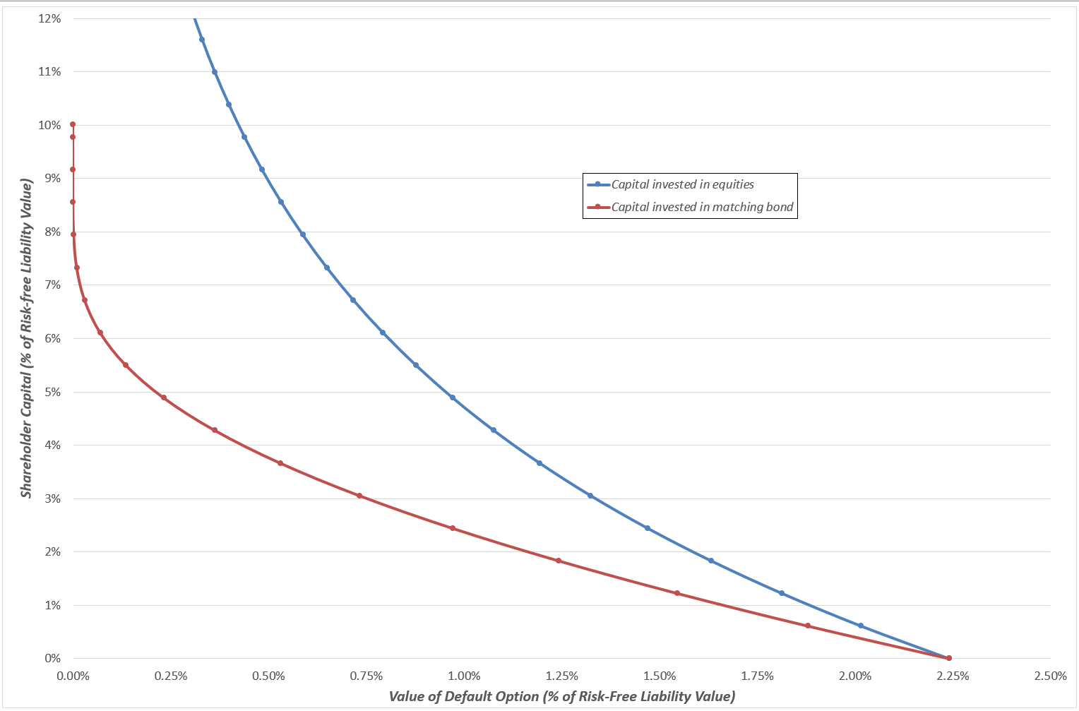
The chart highlights a few intuitive results. In the case of capital being invested in the matching bond, a 10% capital requirement ensures that there is a sufficient total allocation to the matching bond to fully match the liability cashflow, and the default option value is therefore reduced to zero. In the event that no capital is held beyond the basic reserve, the default option value is clearly the same for both capital investment strategies. If some capital is held, then more capital is required to obtain a given default option value when the capital is invested in equities relative to when it is invested in the matching bond.

Note that we have not considered the case where the basic reserve is less than the promised liability cashflow discounted at the risk-free rate (without allowance for the default option). In the current regulatory system of Solvency II, such a reserve may be possible due to a variety of features such as the Matching Adjustment, Volatility Adjustment, and the use of yield curve extrapolation parameters (for the Euro) that are clearly inconsistent with current market levels.

5.      Concluding Thoughts

This note has reflected on the theoretical rationale for solvency capital regulation and has developed a quantitative definition of solvency capital requirements that logically follows from this rationale. This measure of solvency capital has some distinctive features relative to the VaR approach used in Solvency II and the run-off approach that has been used widely in recent actuarial history. In particular, it offers two advantages over these other quantitative definitions for risk-sensitive capital requirements:

·       This definition of solvency capital makes no direct use of ‘real-world’ probabilities. This is philosophically appealing to the social science anti-positivist who cannot subscribe to the idea that these probabilities can be estimated with reliable accuracy or, indeed, are particularly meaningful.

·       The capital measure defines how much of the risky asset return should be passed over to the policyholder in the form of a (fixed) reduction in the premiums charged for the insurance policy (and the example above showed the capital requirements that would be commensurate with a 1% reduction in the premium charged). This measure is therefore a more economically meaningful quantity than an arbitrary percentile level.

However, such a definition is, of course, no panacea. Many of the financial market risks (and non-financial risks such as longevity risk) that are found on insurance balance sheets are not risks for which there are observable traded option prices. As a result, the option valuation exercise described above would need to use a valuation method that heavily relied on real-world probability estimates to generate assumed values for the option prices. But actuaries already regularly make use of such assumptions in the valuation of contingent liabilities such as with-profit guarantees, so this does not present any significant new challenges.

Some may object to the rather invidious-sounding characterisation of insurance firms’ investment risk-taking as an attempted transfer of wealth from policyholder to shareholder. It could be argued that the policyholder benefits from this risk-taking as well as the shareholder – the shareholder shares the prospective proceeds of the risk-taking with policyholders in the form of an up-front (fixed) reduction in the premium for the insurance. So is investment risk-taking actually a win-win? The central point of the above analysis is that it is only right that the policyholder is charged less for fixed promises when the shareholder takes investment risk with the policyholder’s premium. After all, their policy is worth less in the presence of the default risk created by the investment risk (albeit the policyholder may not fully appreciate that fact). Whether policyholders want a cheaper insurance policy that comes with more default risk is an interesting and open question that must ultimately hinge, at least in part, on how such products are sold.

It might also be argued that insurance firms’ investment risk-taking with assets backing insurance liabilities is important for the wider economy. These funds are used to finance critical infrastructure and such like. If all of those assets were invested in risk-free bonds, the argument goes, they will simply make risk-free bonds even more expensive than their current all-time record levels. It could be argued in response that if insurance firms wish to participate in risk-taking in the real economy, they should design insurance products that produce a liability structure that is fit for that purpose. This likely means allowing the policyholder to directly and explicitly participate in the investment returns of the assets (such as in unit-linked or with-profit-style product structures). Meanwhile, de-risking the investment strategy for ‘non-profit’ insurance liabilities would release risk capital, reduce investment management expenses and reduce the material costs of regulatory compliance that are associated with holding those assets under principle-based systems such as Solvency II.

References

Bailey (1862), ‘On the Principles on which the Funds of Life Assurance Societies should be Invested’, Journal of the Institute of Actuaries, Vol. 10, pp. 142-147.

Bride and Lomax (1994), ‘Valuation and Corporate Management in a Non-Life Insurance Company’, Journal of the Institute of Actuaries, Vol. 121, No. 2, pp. 363-440.

CRO Forum (2006), ‘A market cost of capital approach to market value margins’.

Ford et al (1980), ‘Report of the Maturity Guarantees Working Party’, Journal of the Institute of Actuaries, Vol. 107, pp. 103-231.

Haldane and Madouros (2012), “The Dog and the Frisbee”, Proceedings – Economic Policy Symposium – Jackson Hole, pp. 109-159.

Hardy (2006), An Introduction to Risk Measures for Actuarial Applications, Casualty Actuarial Society and Society of Actuaries.

King (2016), The End of Alchemy, Little, Brown.

Turnbull (2017), A History of British Actuarial Thought, Palgrave Macmillan.

Wilkie et al (1990), Continuous Mortality Investigation, Report 10, Institute of Actuaries and Faculty of Actuaries.

[1] For the purposes of this note, when we refer to life assurance business, we do not include with-profit business and unit-linked business.  We are focused on the general account assets.
[2] This is not a new idea, either in corporate finance theory or in the specific context of insurance investment. For an example of discussion of the insurance investment irrelevance proposition in the actuarial literature see Section 6.3 of Bride and Lomax (1994).
[3] There are also other important factors such as the tax treatment of different assets and how the tax treatment that applies to investments held by insurers differs from that which applies to other forms of investor. Such factors are doubtless important, but their economic implications are more straightforward, and in in the interests of brevity the topic of tax is not discussed in this note.
[4] This is another not-new idea. It dates back in the actuarial literature at least as far back as Bailey (1862) (no typo!). See Turnbull (2017) Chapter 3 for a fuller discussion.
[5] See, for example CRO Forum (2006).
[6] Again, see Bride and Lomax (1994), for example.
[7] Ford et al (1980). Again, see Turnbull (2017) for further discussion of this historical episode.
[8] See, for example, Hardy (2006) for a comprehensive introductory treatment in an actuarial context.
[9] I hope to have much more to say about risk measurement and risk management in the presence of deep uncertainty in future writing. Suffice it say for now, this is, of course, not a new topic (see, for example, some of the writings of a fairly diverse bunch such as Hume, Knight, Hayek, Keynes, Popper, Weber, Simon and the actuary Frank Redington). It is a topic that has been increasingly reflected in the thinking of thought-leaders on financial regulation, especially since the Global Financial Crisis. See, for example, Haldane and Madouros (2012) and King (2016).
[10] This argument can be made in many ways and has been (see the writers referred to in Footnote 9). One succinct version: human behaviour depends on knowledge. Future human behaviour will depend, in part, on new knowledge. We cannot say today what that new knowledge is. That’s what will make it new. We therefore cannot predict in a quantifiably accurate sense how social phenomena will behave in the future.
[11] Based on the mortality improvement function published in CMI Report 10, p. 52 and IM(80).
[12] I am not aware that this is not a new idea. But it probably isn’t.